www.slide4math.com

This is my version of explanation. I would suggest you to come up with your own explanation. The best way would be for you to try explain this to somebody else in your own words.

Following is my version of explanation, but this is just an example. You may come up with a better version.

DFT (Digital Fourier Transform) - Truncated Rectangular Wave

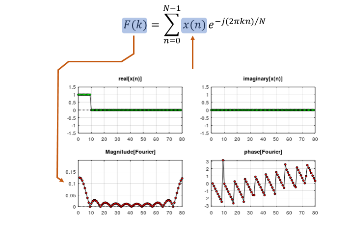
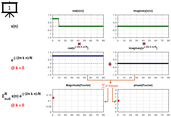
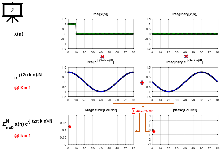
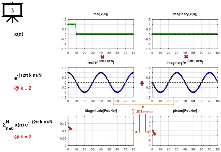
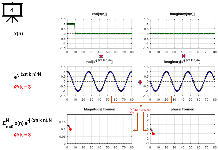
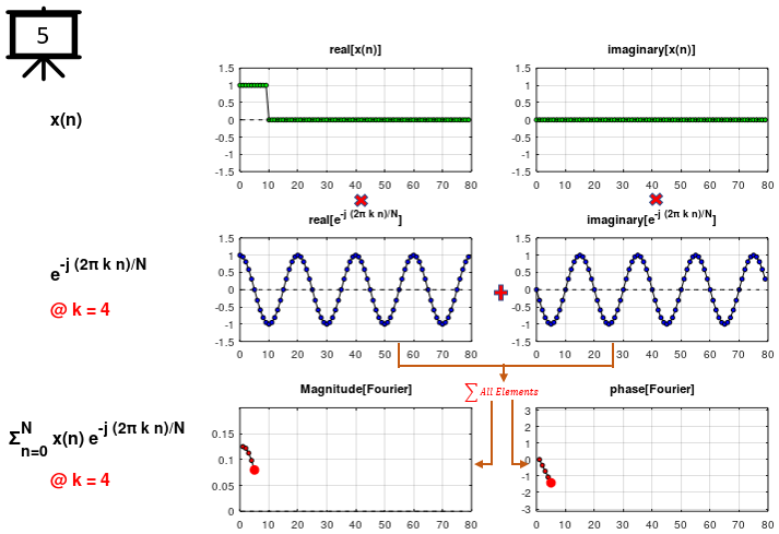
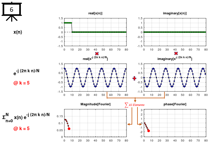
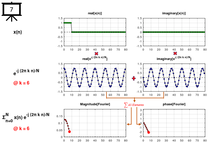
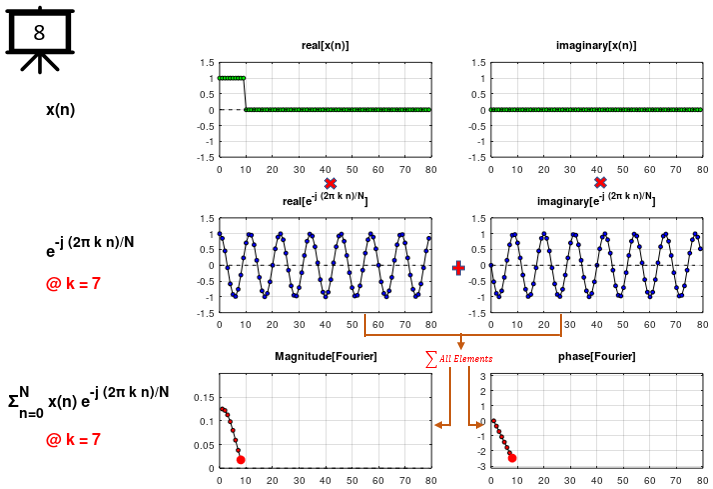
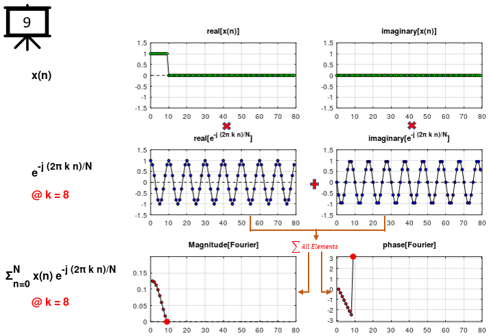
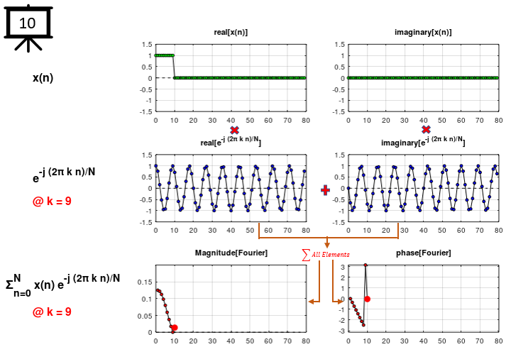
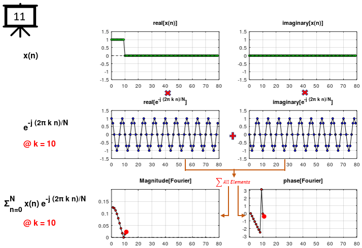
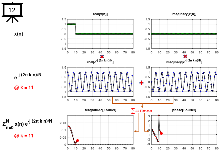
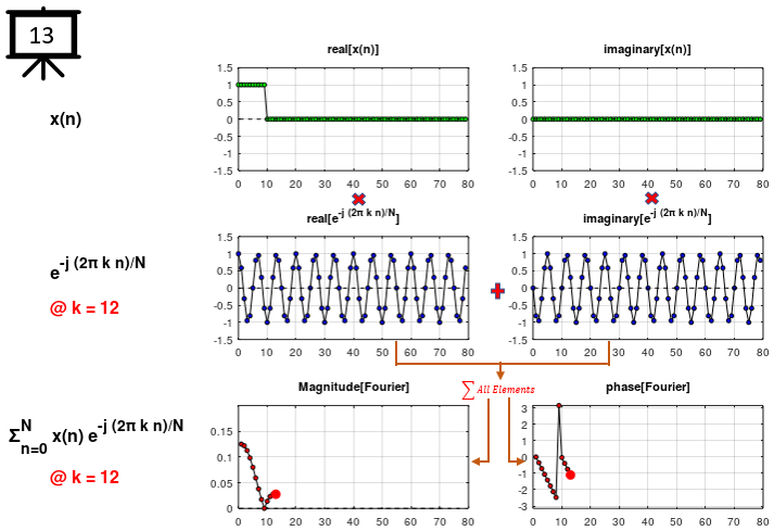
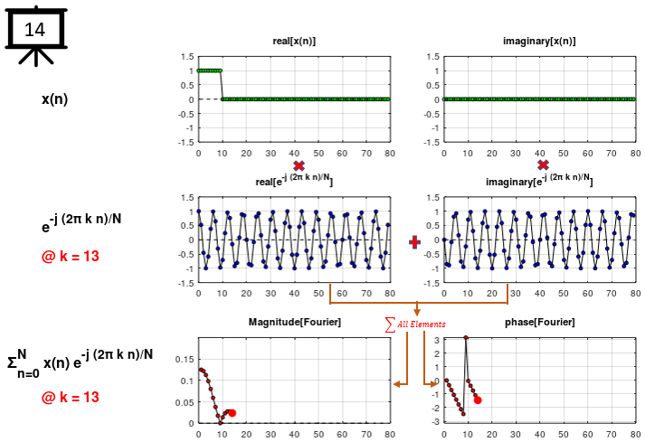
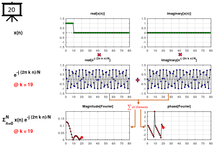
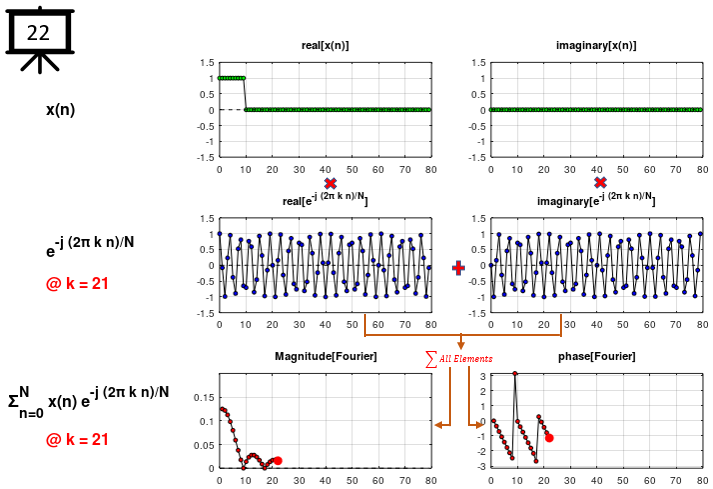
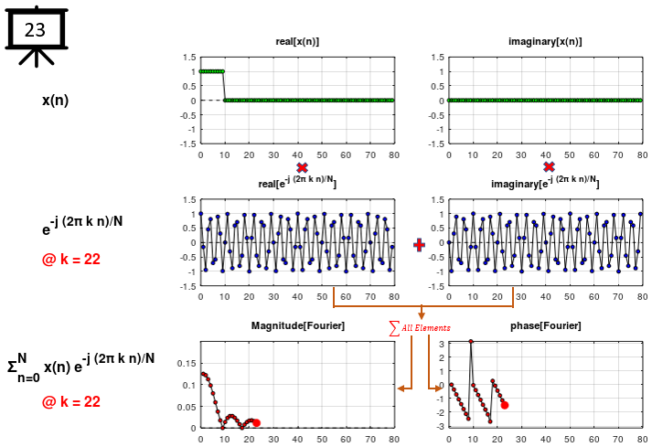
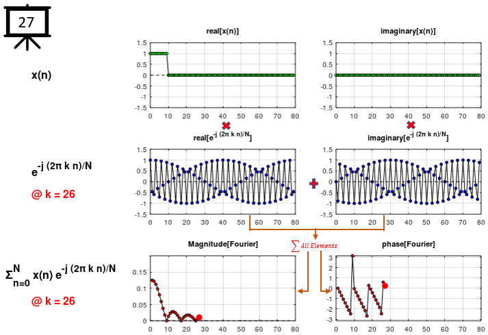
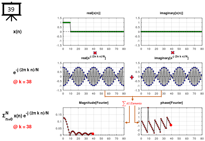
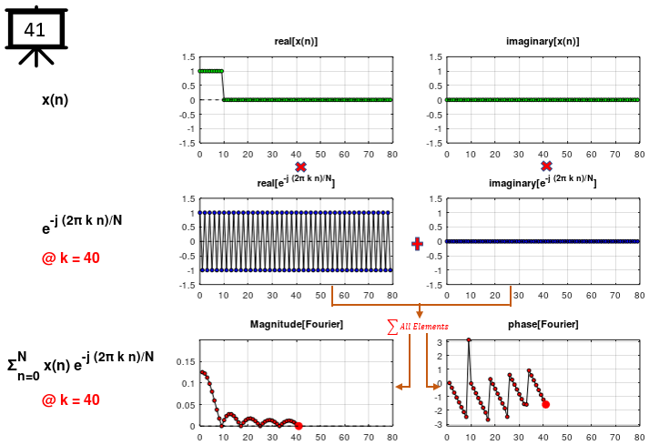
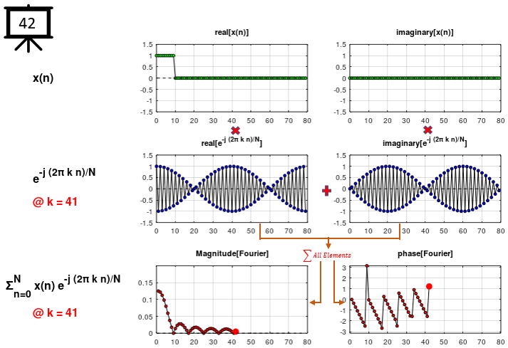
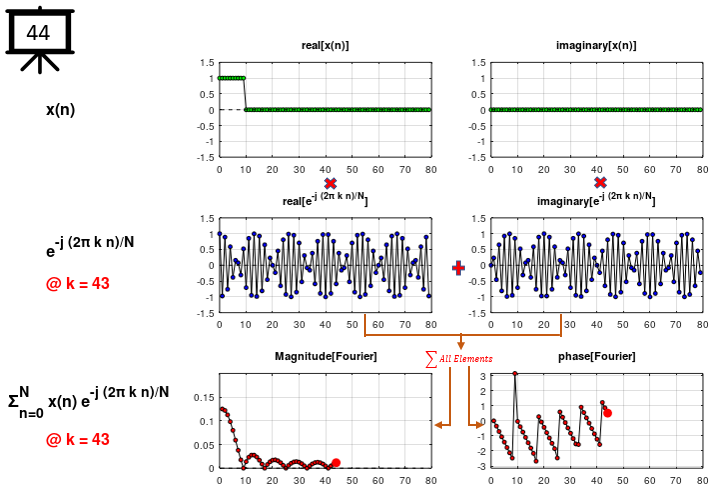
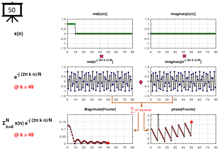
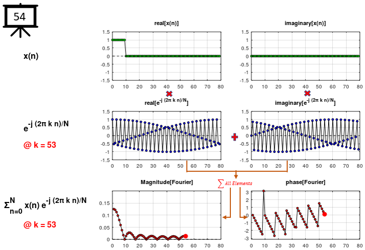
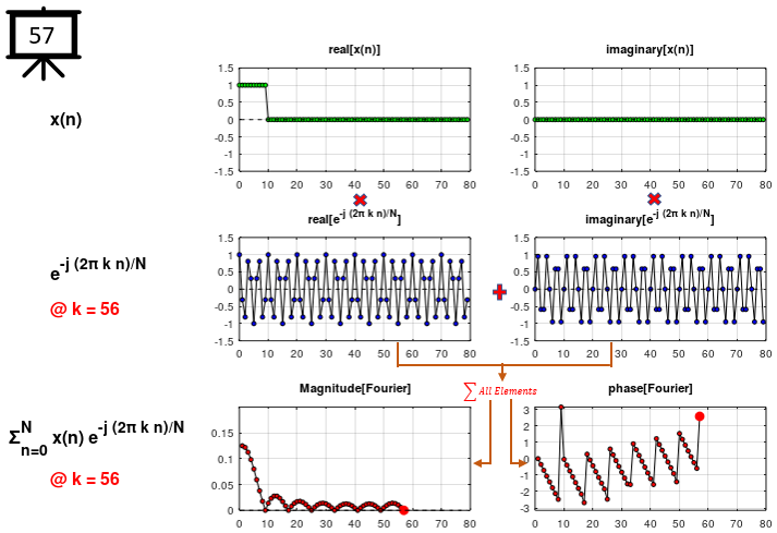
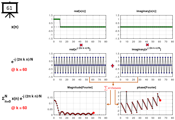
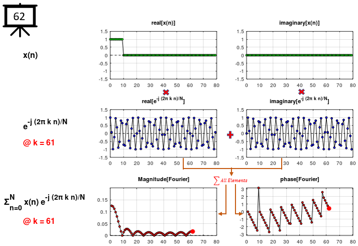
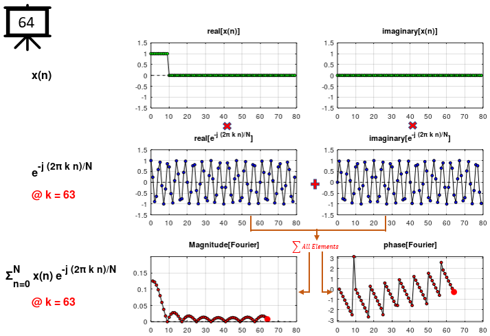
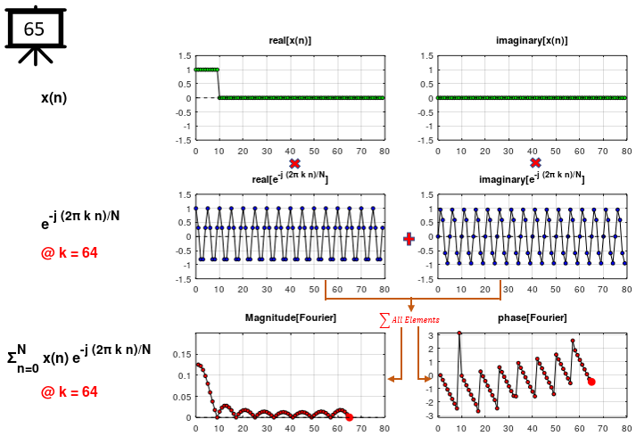
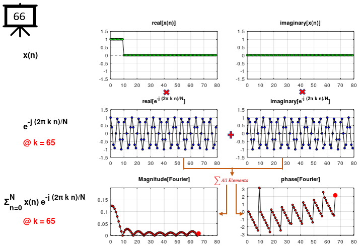
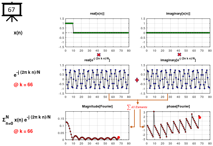
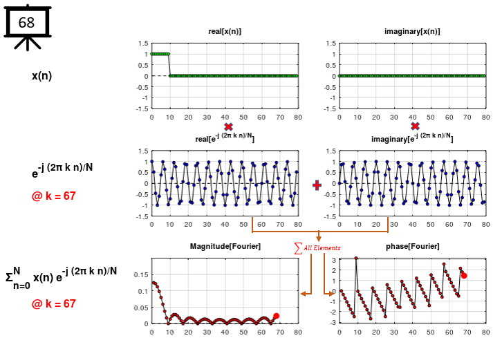
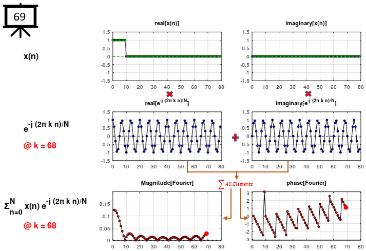
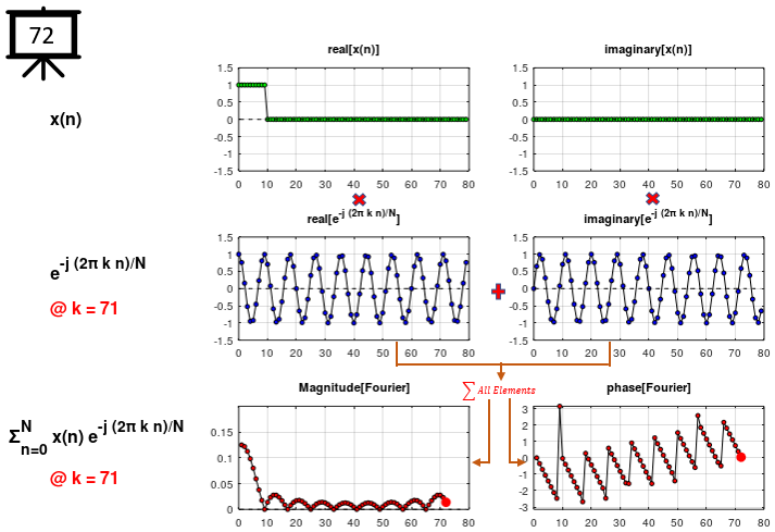
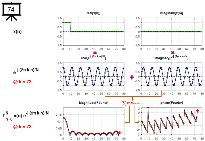
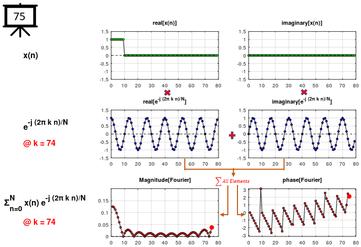
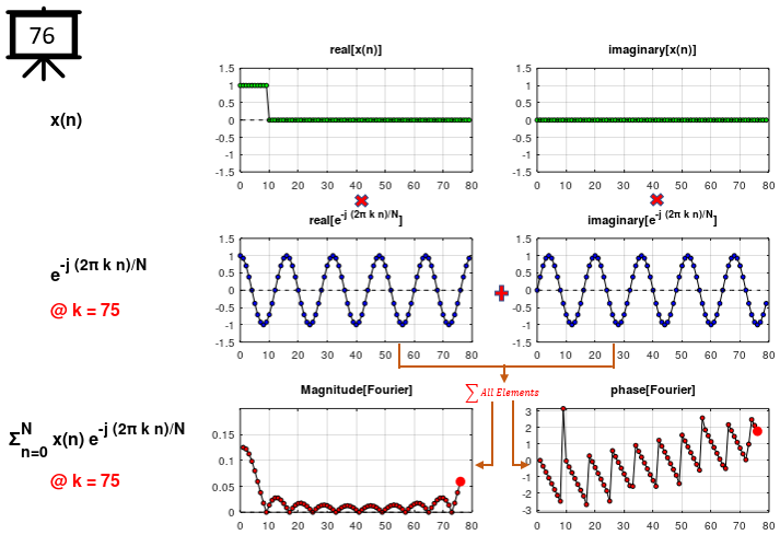
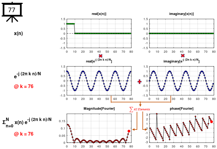
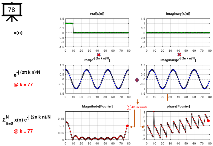
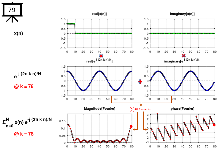
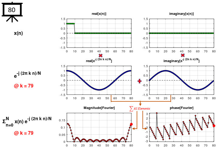
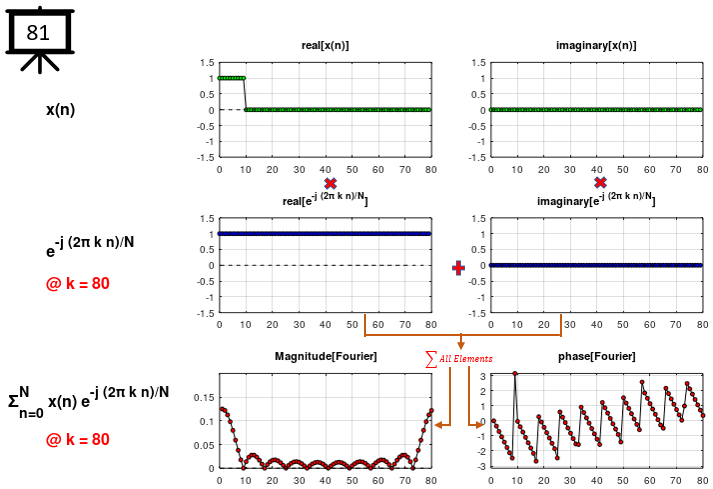
Followings are the code that I wrote in Octave to creates all the plots shown in this page. You may copy these code and play with these codes. Change variables and try yourself until you get your own intuitive understanding.

< Code 1 >

f = 4;

ph = 0;

x = linspace(-pi,pi,80);

sig = sin(f .* x);

pLength = 10;

for i = 1:length(sig)

  if(i <= pLength)

      sig(i) = 1.0;

  else

      sig(i) = 0.0;

  end    

end  

n = 0:length(x)-1;

N = length(n);

i = 80;

ft = []

for k = 0:i

  e_k = exp(-j*2*pi*k*n ./ N);

  sig_re = real(sig);

  sig_im = imag(sig);

  e_k_re = real(e_k);

  e_k_im = imag(e_k);

  sig_c = sig_re + j .* sig_im;

  e_k_c = e_k_re + j .* e_k_im;

  ft_k = sum(sig_c .* e_k_c)/N;

  ft = [ft ft_k];

end

hFig = figure(1,'Position',[300 300 800 500]);

sig_y = [-1.5 1.5];

ek_y = [-1.5 1.5];

ft_y = [0 0.2];

ft_phase_y = [-pi pi];

subplot(3,5,1);

axis([0 1 0 1]);

text(-0.5,0.5,'x(n)','FontSize',16,'fontweight','bold');

set(gca,'Visible','off')

subplot(3,5,[2 3]);

hold on;

plot(n,sig_re,'ko-','MarkerFaceColor',[0 1 0],'MarkerSize',4);

plot(n,zeros(1,length(n)),'k--');

ylim(sig_y);

set(gca,'xtick',[0 10 20 30 40 50 60 70 80]);

grid on;

title('real[x(n)]');

box on;

hold off;

subplot(3,5,[4 5]);

hold on;

plot(n,sig_im,'ko-','MarkerFaceColor',[0 1 0],'MarkerSize',4);

plot(n,zeros(1,length(n)),'k--');

ylim(sig_y);

title('imaginary[x(n)]');

set(gca,'xtick',[0 10 20 30 40 50 60 70 80]);

grid on;

box on;

hold off;

subplot(3,5,6);

axis([0 1 0 1]);

text(-0.5,0.7,'e^{-j (2\pi k n)/N}','FontSize',16,'fontweight','bold');

tStr = sprintf('@ k = %d',i);

text(-0.5,0.3,tStr,'FontSize',16,'fontweight','bold','color','red');

set(gca,'Visible','off')

subplot(3,5,[7 8]);

hold on;

plot(n,e_k_re,'ko-','MarkerFaceColor',[0 0 1],'MarkerSize',4);

plot(n,zeros(1,length(n)),'k--');

ylim(ek_y);

title('real[e^{-j (2\pi k n)/N}]');

set(gca,'xtick',[0 10 20 30 40 50 60 70 80]);

grid on;

box on;

hold off;

subplot(3,5,[9 10]);

hold on;

plot(n,e_k_im,'ko-','MarkerFaceColor',[0 0 1],'MarkerSize',4);

plot(n,zeros(1,length(n)),'k--');

ylim(ek_y);

title('imaginary[e^{-j (2\pi k n)/N}]');

set(gca,'xtick',[0 10 20 30 40 50 60 70 80]);

grid on;

box on;

hold off;

subplot(3,5,11);

axis([0 1 0 1]);

text(-1.0,0.7,'\Sigma_{n=0}^{N} x(n) e^{-j (2\pi k n)/N}','FontSize',16,'fontweight','bold');

tStr = sprintf('@ k = %d',i);

text(-0.5,0.3,tStr,'FontSize',16,'fontweight','bold','color','red');

set(gca,'Visible','off')

subplot(3,5,[12 13]);

hold on;

plot(abs(ft),'ko-','MarkerFaceColor',[1 0 0],'MarkerSize',4);

plot(i+1,abs(ft(end)),'ro','MarkerFaceColor',[1 0 0],'MarkerSize',8);

plot(n,zeros(1,length(n)),'k--');

xlim([0 length(n)]);

ylim(ft_y);

title('Magnitude[Fourier]');

set(gca,'xtick',[0 10 20 30 40 50 60 70 80]);

grid on;

box on;

hold off;

subplot(3,5,[14 15]);

hold on;

plot(arg(ft),'ko-','MarkerFaceColor',[1 0 0],'MarkerSize',4);

plot(i+1,arg(ft(end)),'ro','MarkerFaceColor',[1 0 0],'MarkerSize',8);

plot(0,zeros(1,length(n)),'k--');

xlim([0 length(n)]);

ylim(ft_phase_y);

title('phase[Fourier]');

set(gca,'xtick',[0 10 20 30 40 50 60 70 80]);

grid on;

box on;

hold off;