www.slide4math.com

This is my version of explanation. I would suggest you to come up with your own explanation. The best way would be for you to try explain this to somebody else in your own words.

Following is my version of explanation, but this is just an example. You may come up with a better version.

A very special form of exponential function.

You all may know that the exponential function is one of the most famous form of the exponential form. I think one of the major reasons on why the exponential function has become such a famous one would be due to this special form of exponential function as shown on this page.

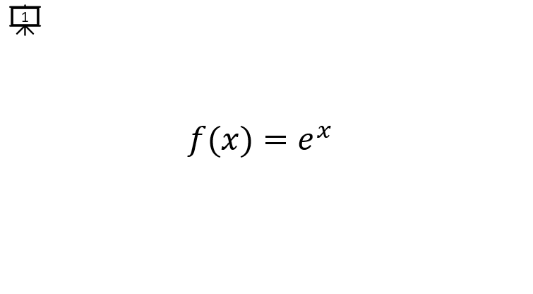
It is the special form of the exponential form that use the special constant 'e' as the base of the function.

[Slide 1] This is the form of a special exponential function that we will look into on this slides.

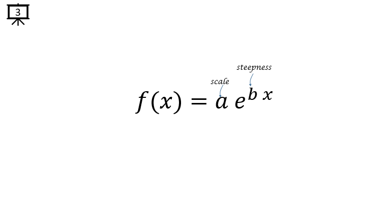
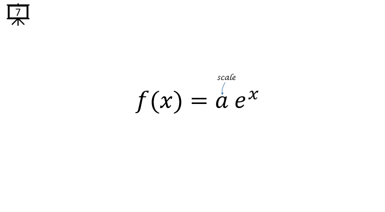
[Slide 2] As in any function, you can scale this exponential function as shown here.

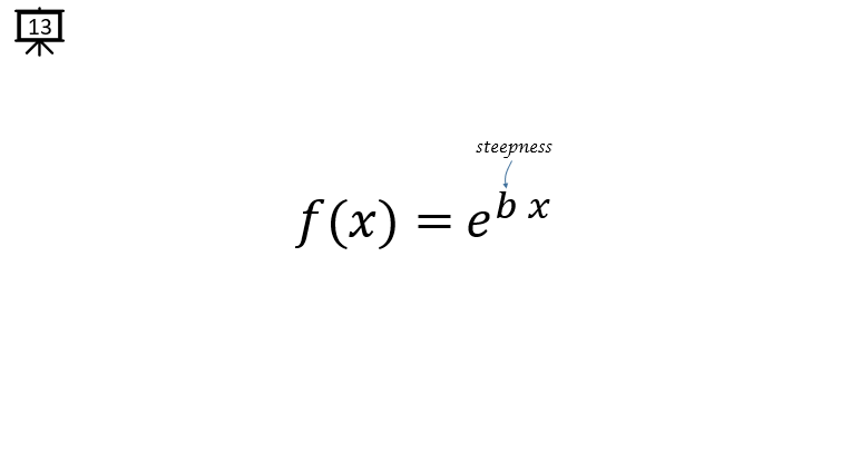
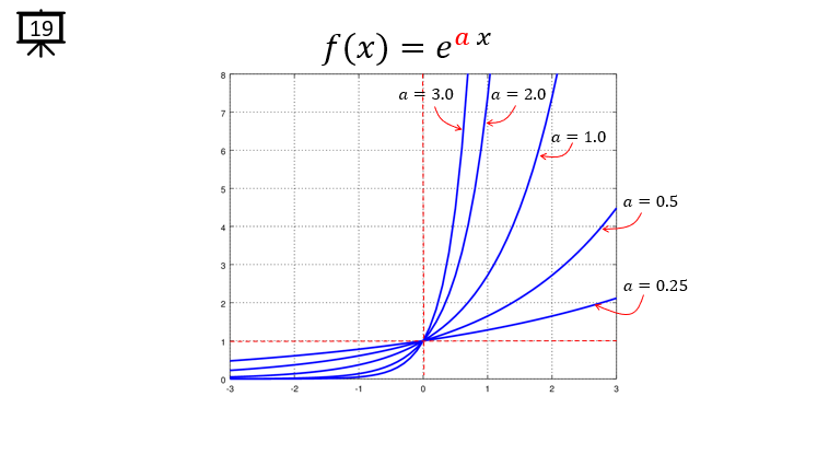
[Slide 3] You can change the steepness of the function (another type of scaling) using the parameter 'b' as shown here.

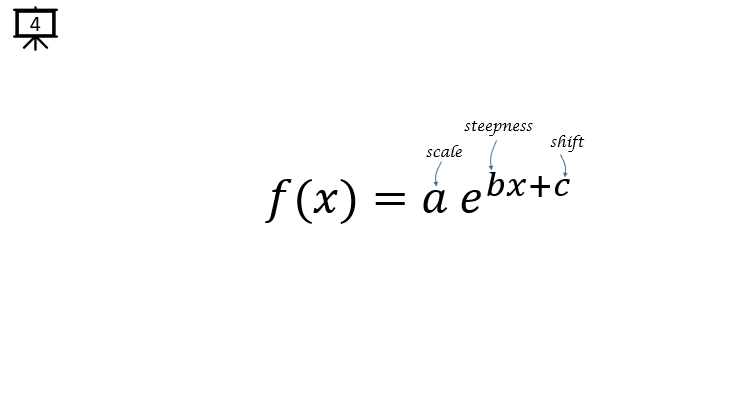
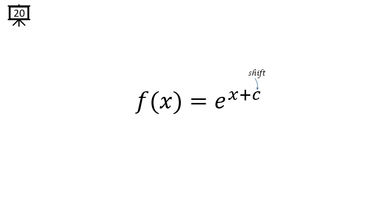
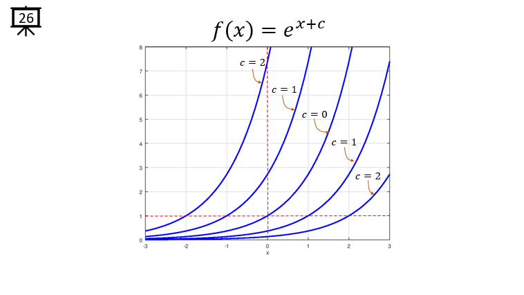
[Slide 4] You can shift the function along x axis using the parameter 'c' as shown here.

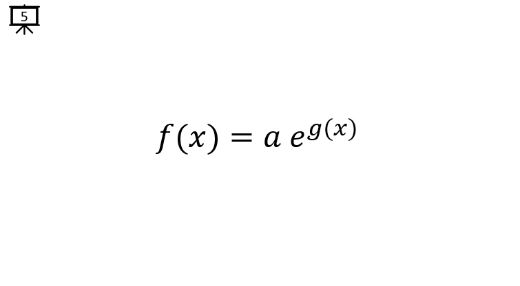
[Slide 5] In real application of the exponential function, the exponent part would take more complicated form (the exponent itself can be a function) as shown here. In engineering, this would be the most frequently used form of the exponential function.

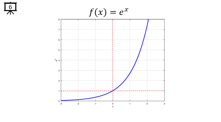
[Slide 6] This is the graph of the basic form. Check how the graph changes in following slides.

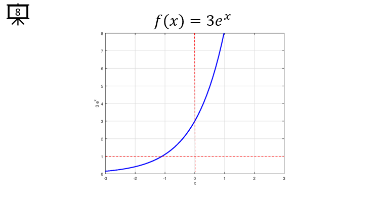
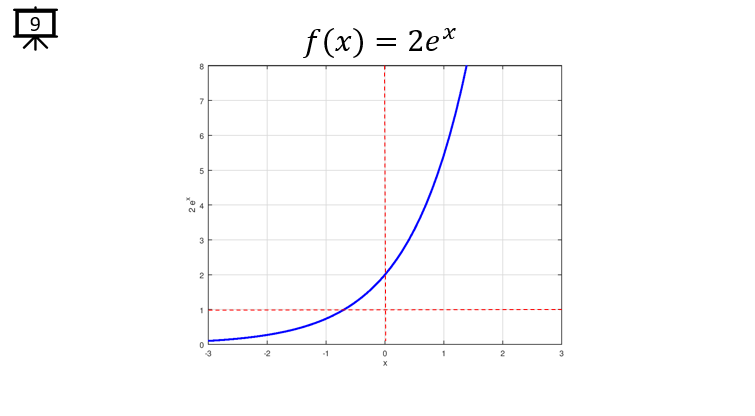
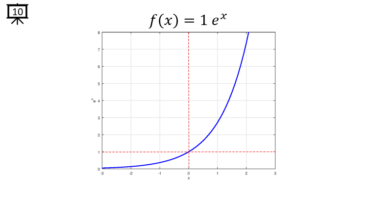
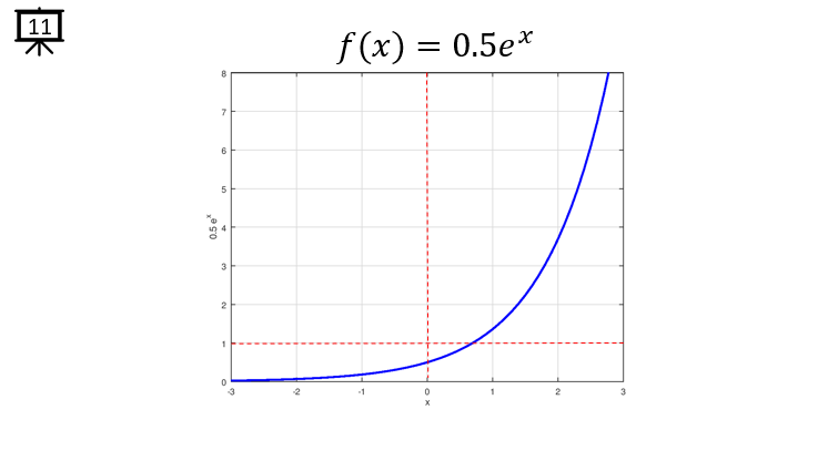
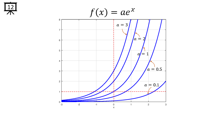
[Slide 7~12] Now let's see how graph changes as the scaling factor changes.

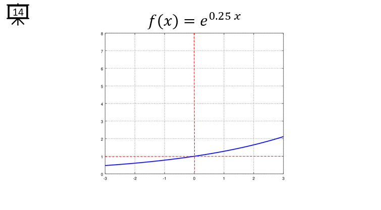
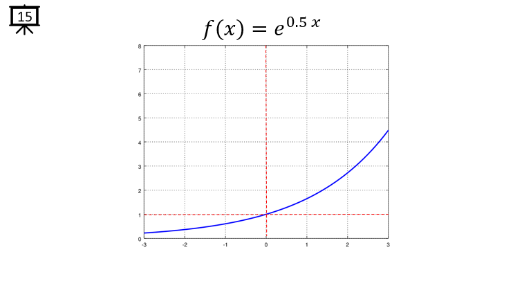
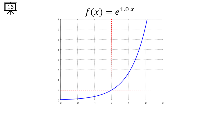
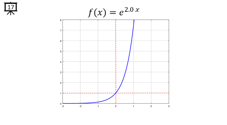
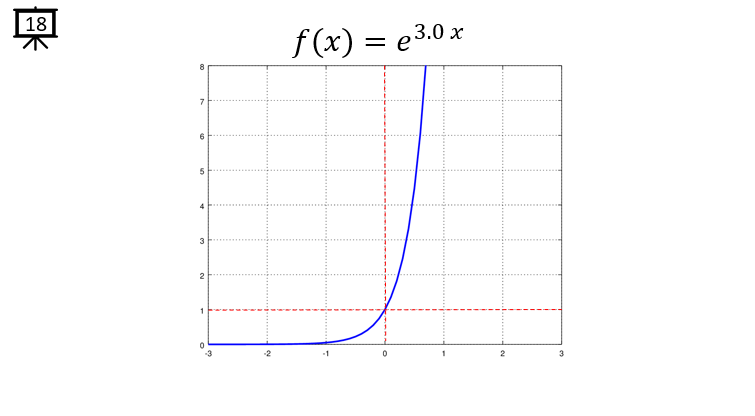
[Slide 13~19] This shows the case of scaling the indepenent variable 'x'. Compare this with [Slide 7~12] and see how they are different from each other.

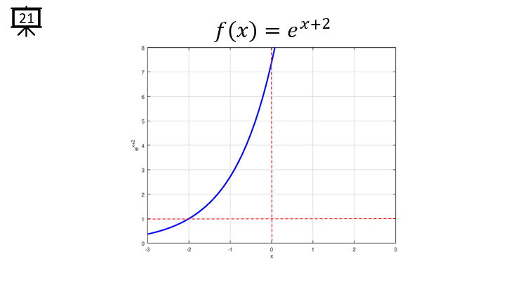
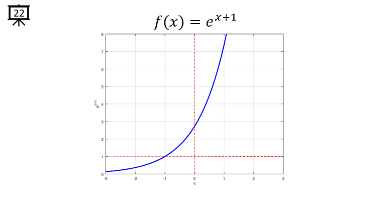
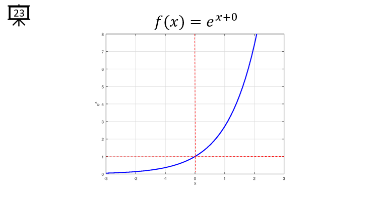
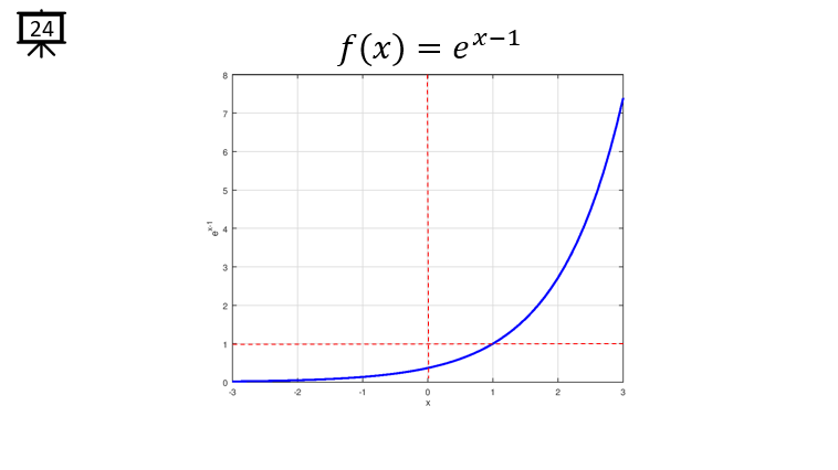
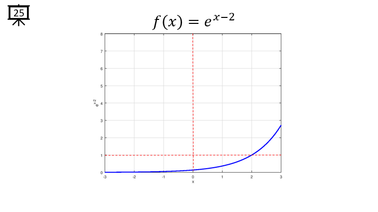
[Slide 20~26] This shows you the case of shifting the exponential graph.

Followings are the code that I wrote in Octave to creates all the plots shown in this page. You may copy these code and play with these codes. Change variables and try yourself until you get your own intuitive understanding.

< Code 1 >

x = -3:0.1:3;

a = 1;

b = 1.0;

c = 0;

y = a * exp(b * x + c);

plot(x,y,'b-','Linewidth',2);

ylim([0 8]);

set(gca,'ytick',0:1:8);

grid on;

< Code 2 >

x = -3:0.1:3;

aList = [1 2 3];

hold on;

for a = aList

y = a * exp(b * x + c);

plot(x,y,'b-','Linewidth',2);

ylim([0 8]);

end

hold off;

set(gca,'ytick',0:1:8);

grid on;

< Code 3 >

x = -3:0.1:3;

bList = [0.25 0.5 1.0 2.0 3.0];

hold on;

for b = bList

y = exp(b .* x);

plot(x,y,'b-','Linewidth',2);

ylim([0 8]);

end

hold off;

set(gca,'ytick',0:1:8);

grid on;